Kyo Harada — Visage AI / Data Scientist
On-device skin analytics with finance-grade pipelines—CoreML optimization, RAG systems, and real-time evaluation.
- −75% model size
- 3× inference
- −60% RAM
- <5% Δ accuracy
Core Capabilities
On-device Skin Scoring
CoreML-optimized models for real-time skin analysis with privacy-first design.
Evaluation Dashboard
RAG/LLM audit with reproducible benchmarks and actionable recommendations.
Privacy by Design
On-device processing so data never leaves the user's device.
Financial Review of Pendragon PLC
This is a modified version of the report for Corporate Finance in Bath Full Time MBA Class of 2020.
Financial Review of Pendragon PLC
Introduction
“Cash is fact, profit is opinion” was argued by The Economist because such accounting figures can be manipulated conveniently (Anonymous, 1997). This might imply the framework to analyze the company is changing, however, the importance of valuation and analysis itself may be stable. This report will review of Pendragon PLC (PDG.L) in terms of their financial performance, position and capability to generate cash flow. In addition, the enterprise value will be calculated using discount cash flow method (DFC) and therefore, the figure will be compared with their market value.
Review of Financial Performance
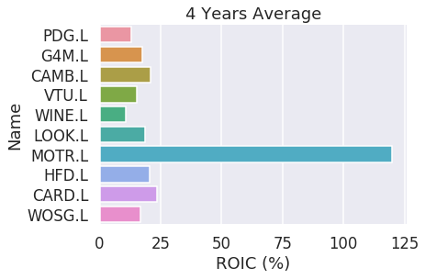
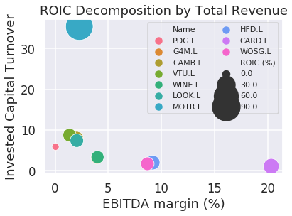
From the investor’s point of view, the performance of company can be represented by return on invested capital (ROIC). This is mainly because ROIC describe how much the company generate the cash flow using capital in which the finance providers invested such as equity and debt (Watson and Head, 2019). In general, the cash flow is indicated by net operating profit less adjusted taxes (McKinsey & Company, 2010). However, this report uses Earnings Before Interest Taxes Depreciation and Amortization (EBITDA) owing to the fact that EBITDA can be directly extracted from Income Statement which means to be more reliable than the processed one. The Figure 1 show 4 years average ROIC of PDG.L and the major competitors , which the firm can be the second least valuable for the investors because if their investment was used to the competitors or other assets, they would earn more money. Moreover, the ROIC of PDG.L was 0.24% in 2018, which meant not only the least valuable firm but also approximately 13% smaller than its average. ROIC could be decomposed in terms of profitability and efficiency using mainly EBITA Margin and Invested Capital Turnover respectively (ibid). The perspective of cost structure is also important and is represented by two figures which are sales cost ratio and selling, general & administrative (SGA) ratio, however, these number of PDG.L was almost stable for 4 years (ibid). Therefore, Figure 2 show ROIC decomposition by profitability and efficiency. This figure indicates PDG.L has the lower profitability and efficiency than competitors, in contrast, firms with larger ROIC has either profitability or efficiency then both cannot hold at the same time in this industry which is retail and repair of used and new cars. What is the main cause of low ROIC can be recognized to see ROIC trees (Figure 3 and 4). These trees show EBITDA margin, fixed asset turnover and accounts payable turnover of PDG.L are significantly lower than the competitors average. Relatively low EBITDA margin means they might make less effort to cut operating expenses (Investopedia, 2019). Less fixed asset turnover signifies their fixed-asset investments management can be smaller effective (ibid). Lower accounts payable turnover connotes there can be smaller amount cash flow to pay their short-term obligations (ibid).


Review of Financial Position
There are two aspects to analyze financial position of the firm, which are liquidity and gearing (coverage). The major indicators of liquidity are quick rate and current rate. In comparison with the average of competitors, these ratios are 17% (0.97) and 28% (0.22) lower respectively. This means PDG.L has less capability to pay short term obligations and therefore they are more likely to be bankruptcy (Investopedia, 2019). Gearing is represented by capital gearing, debt-to-equity and interest coverage ratio. They have moderate capital gearing (0.25) and debt-to-equity (4.10) because these difference with the average of competitors are 10% and 5% higher, however, interest coverage of them (2.39) is 84% smaller. This means their interest expense can be quite larger than their earnings therefore the likelihood of bankruptcy might be higher and this statement is supported both liquidity and gearing (ibid).
Review of the cash generation
Most investors are interested in the structure and capability to earn free cash flow. This is because the value of company can be driven by cash flow which is created their ROIC and revenue growth (McKinsey & Company, 2010). Free cash flow of PDG.L has been negative for 5 years, however, operating cash flow has been positive for the same period and larger than the average . This means capital expenditure of them has been considerably larger than operating cash flow . This was mainly due to the fact that they recognized a significant impairment of £88.8M against the carrying value of goodwill in a number of its Cash Generating Units (AR18p77). Therefore, if they did not recognize the impairment, free cash flow would £34.6M, which means they might have the capability to earn cash flow because free cash flow exclude goodwill was positive and such impairment is less likely to be happen.
DCF Based Valuation
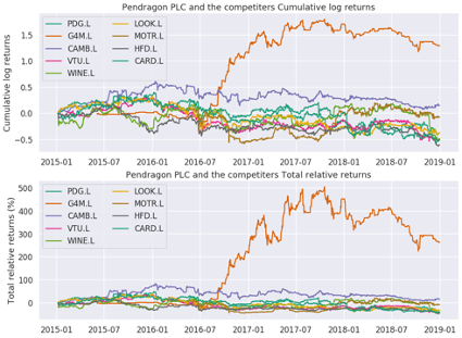
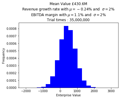
There is the history of stock price in Figure 5, which indicate after global recession in 2008, although until 2016 the price had been recovering, it is decreasing again and therefore enterprise value as market capitalization (MC) is also declining to £158.97M as of 2019 according to Yahoo! Finance. This decrease could recognize the historical cumulative log return and total relative one of stock price in Figure 6. However, some people argue that MC do not represent the value of firm. There are three approaches to evaluate the company which are income, cost and market approach mainly including MC (McKinsey & Company, 2010). Discount cash flow method can be the most popular income approach valuation one, which the estimated future free cash flows multiplying weighted average cost of capital (WACC) as a discount factor and then those discounted free cash flows is summed up is considered as enterprise value (ibid). Assumed CAPM theory hold, WACC is calculated as 3.81% which might mean the investor lost the opportunity to earn more money investing other assets such as stocks or bonds due to the fact that average ROIC is 12.92%. The determination of value drivers is important to estimate future free cash flow. In general, some of key drivers are revenue growth, EBITDA margin and tax rate. As a base line scenario, those are assumed as compound average growth rate (CAGR, -0.24% ), weighted average EBITDA margin (1.10%) and British tax rate (19% in 2019 and 17% from 2020) respectively. Therefore, CAGR estimated future 5 years revenue (2019-2023) and then EBITDA was calculated by multiplying the revenue with EBITDA margin. Assumed percentage of depreciation and amortization against revenue is constant and equal to the figure in 2018 (0.66%), the future depreciation and amortization was earned to multiply the revenue with the percentage. The future earnings before interest and taxes (EBIT) was reckoned the EBITDA minus depreciation and amortization. Future free cash flow (FCF) was estimated the EBIT minus operating cash tax which EBIT multiplied tax rate. Finally, the enterprise value was £498.04M owing to the fact that those 5 years FCF was discounted by WACC and totaled. In comparison with market cap, the estimated value was almost 3 times higher which means the current market value can be undervalued by market participants. However, the base line of DCF method might be unreliable because of the uncertainty of prediction for key drivers primary revenue growth and therefore it should be mitigated to use some feasible scenarios which should be averaged weightily based on it’s feasibility or to adapt Monte Carlo simulation (MC). As a result of the adaption (see figure 7), the enterprise value was £430.04M, which meant several scenarios were smoothened using two normal distributions for revenue growth and EBITDA margin, both of which have 2% standard deviation.

Conclusion
This report has reviewed PDG.L’s financial conditions and estimated their enterprise value. As a result of the review, EBITDA margin, fixed asset and account payable turnover were considerably smaller than major competitors. In addition, in terms of liquidity and gearing, they might be lower capability to pay short term debt. According to their cash generation, they have relatively large operating cash flow, however, capital expenditure was higher than their cash earning ability from business. This might mean lower turnovers lead to lower liquidity and gearing, therefore, capital expenditure may become larger and thus their free cash flow earning ability become weaker. This can be supported by that estimated enterprise value with DCF and MC (£430.04M) was approximately 3 times larger than their market cap. This may mean market participants are significantly concerned to their capability to earn free cash flow more than assumed and estimated in this report. The valuation did not consider inflation, foreign currency, pension obligation effects and other factors to affect the value, however, these should be done so to calculate the value more precisely.
Reference
- Anonymous, 1997. A star to sail by? The Economist, 344(8028), pp.53–55.
- Cambria Automobiles PLC. (CAMB.L), 2019. Balance Sheet. Yahoo!Finance. Retrieved from: https://finance.yahoo.com/quote/CAMB.L/balance-sheet?p=CAMB.L [Accessed 20 December 2019].
- Cambria Automobiles PLC. (CAMB.L), 2019. Income statement. Yahoo!Finance. Retrieved from: https://finance.yahoo.com/quote/CAMB.L/financials?p=CAMB.L [Accessed 20 December 2019].
- Cambria Automobiles PLC. (CAMB.L), 2019. Key Statistics. Yahoo!Finance. Retrieved from: https://finance.yahoo.com/quote/CAMB.L/key-statistics?p=CAMB.L [Accessed 20 December 2019].
- Cambria Automobiles PLC. (CAMB.L), 2019. Statement of Cash Flows. Yahoo!Finance. Retrieved from: https://finance.yahoo.com/quote/CAMB.L/cash-flow?p=CAMB.L [Accessed 20 December 2019].
- Card Factory PLC. (CARD.L), 2019. Balance Sheet. Yahoo!Finance. Retrieved from: https://finance.yahoo.com/quote/CARD.L/balance-sheet?p=CARD.L [Accessed 20 December 2019].
- Card Factory PLC. (CARD.L), 2019. Income statement. Yahoo!Finance. Retrieved from: https://finance.yahoo.com/quote/CARD.L/financials?p=CARD.L [Accessed 20 December 2019].
- Card Factory PLC. (CARD.L), 2019. Key Statistics. Yahoo!Finance. Retrieved from: https://finance.yahoo.com/quote/CARD.L/key-statistics?p=CARD.L [Accessed 20 December 2019].
- Card Factory PLC. (CARD.L), 2019. Statement of Cash Flows. Yahoo!Finance. Retrieved from: https://finance.yahoo.com/quote/CARD.L/cash-flow?p=CARD.L [Accessed 20 December 2019].
- Financial Times (FT), 2019. Ten year government bond spreads. [online] Available from: https://markets.ft.com/data/bonds/government-bonds-spreads [Accessed 20 December 2019].
- Gear4music Holdings PLC. (G4M.L), 2019. Balance Sheet. Yahoo!Finance. Retrieved from: https://finance.yahoo.com/quote/G4M.L/balance-sheet?p=G4M.L [Accessed 20 December 2019].
- Gear4music Holdings PLC. (G4M.L), 2019. Income statement. Yahoo!Finance. Retrieved from: https://finance.yahoo.com/quote/G4M.L/financials?p=G4M.L [Accessed 20 December 2019].
- Gear4music Holdings PLC. (G4M.L), 2019. Key Statistics. Yahoo!Finance. Retrieved from: https://finance.yahoo.com/quote/G4M.L/key-statistics?p=G4M.L [Accessed 20 December 2019].
- Gear4music Holdings PLC. (G4M.L), 2019. Statement of Cash Flows. Yahoo!Finance. Retrieved from: https://finance.yahoo.com/quote/G4M.L/cash-flow?p=G4M.L [Accessed 20 December 2019].
- Halfords Group plc. (HFD.L), 2019. Balance Sheet. Yahoo!Finance. Retrieved from: https://finance.yahoo.com/quote/HFD.L/balance-sheet?p=HFD.L [Accessed 20 December 2019].
- Halfords Group plc. (HFD.L), 2019. Income statement. Yahoo!Finance. Retrieved from: https://finance.yahoo.com/quote/HFD.L/financials?p=HFD.L [Accessed 20 December 2019].
- Halfords Group plc. (HFD.L), 2019. Key Statistics. Yahoo!Finance. Retrieved from: https://finance.yahoo.com/quote/HFD.L/key-statistics?p=HFD.L [Accessed 20 December 2019].
- Halfords Group plc. (HFD.L), 2019. Statement of Cash Flows. Yahoo!Finance. Retrieved from: https://finance.yahoo.com/quote/HFD.L/cash-flow?p=HFD.L [Accessed 20 December 2019].
- Investopedia, 2019. Accounts Payable Turnover Ratio Definition. [online] Available from: https://www.investopedia.com/terms/a/accountspayableturnoverratio.asp [Accessed 20 December 2019].
- Investopedia, 2019. Debt-To-Equity Ratio – D/E. [online] Available from: https://www.investopedia.com/terms/d/debtequityratio.asp [Accessed 20 December 2019].
- Investopedia, 2019. EBITDA Margin. [online] Available from: https://www.investopedia.com/terms/e/ebitda-margin.asp [Accessed 20 December 2019].
- Investopedia, 2019. Fixed Asset Turnover Ratio Definition. [online] Available from: https://www.investopedia.com/terms/f/fixed-asset-turnover.asp [Accessed 20 December 2019].
- Investopedia, 2019. How Do I Use the CAPM to Determine Cost of Equity?. [online] Available from: https://www.investopedia.com/ask/answers/022515/how-do-i-use-capm-capital-asset-pricing-model-determine-cost-equity.asp [Accessed 20 December 2019].
- Investopedia, 2019. How to Analyze a Company’s Financial Position. [online] Available from: https://www.investopedia.com/articles/fundamental/04/063004.asp [Accessed 20 December 2019].
- Investopedia, 2019. Interest Coverage Ratio Definition. [online] Available from: https://www.investopedia.com/terms/i/interestcoverageratio.asp [Accessed 20 December 2019].
- Investopedia, 2019. Quick Ratio Definition. [online] Available from: https://www.investopedia.com/terms/q/quickratio.asp [Accessed 20 December 2019].
- Investopedia, 2019. Weighted Average Cost of Capital – WACC. [online] Available from: https://www.investopedia.com/terms/w/wacc.asp [Accessed 20 December 2019].
- Lookers PLC. (LOOK.L), 2019. Balance Sheet. Yahoo!Finance. Retrieved from: https://finance.yahoo.com/quote/LOOK.L/balance-sheet?p=LOOK.L [Accessed 20 December 2019].
- Lookers PLC. (LOOK.L), 2019. Income statement. Yahoo!Finance. Retrieved from: https://finance.yahoo.com/quote/LOOK.L/financials?p=LOOK.L [Accessed 20 December 2019].
- Lookers PLC. (LOOK.L), 2019. Key Statistics. Yahoo!Finance. Retrieved from: https://finance.yahoo.com/quote/LOOK.L/key-statistics?p=LOOK.L [Accessed 20 December 2019].
- Lookers PLC. (LOOK.L), 2019. Statement of Cash Flows. Yahoo!Finance. Retrieved from: https://finance.yahoo.com/quote/LOOK.L/cash-flow?p=LOOK.L [Accessed 20 December 2019].
- McKinsey & Company, 2010. VALUATION. FIFTH EDITION. John Wiley & Sons, Inc.
- Motorpoint Group PLC. (MOTR.L), 2019. Balance Sheet. Yahoo!Finance. Retrieved from: https://finance.yahoo.com/quote/MOTR.L/balance-sheet?p=MOTR.L [Accessed 20 December 2019].
- Motorpoint Group PLC. (MOTR.L), 2019. Income statement. Yahoo!Finance. Retrieved from: https://finance.yahoo.com/quote/MOTR.L/financials?p=MOTR.L [Accessed 20 December 2019].
- Motorpoint Group PLC. (MOTR.L), 2019. Key Statistics. Yahoo!Finance. Retrieved from: https://finance.yahoo.com/quote/MOTR.L/key-statistics?p=MOTR.L [Accessed 20 December 2019].
- Motorpoint Group PLC. (MOTR.L), 2019. Statement of Cash Flows. Yahoo!Finance. Retrieved from: https://finance.yahoo.com/quote/MOTR.L/cash-flow?p=MOTR.L [Accessed 20 December 2019].
- Naked Wines PLC. (WINE.L), 2019. Balance Sheet. Yahoo!Finance. Retrieved from: https://finance.yahoo.com/quote/WINE.L/balance-sheet?p=WINE.L [Accessed 20 December 2019].
- Naked Wines PLC. (WINE.L), 2019. Income statement. Yahoo!Finance. Retrieved from: https://finance.yahoo.com/quote/WINE.L/financials?p=WINE.L [Accessed 20 December 2019].
- Naked Wines PLC. (WINE.L), 2019. Key Statistics. Yahoo!Finance. Retrieved from: https://finance.yahoo.com/quote/WINE.L/key-statistics?p=WINE.L [Accessed 20 December 2019].
- Naked Wines PLC. (WINE.L), 2019. Statement of Cash Flows. Yahoo!Finance. Retrieved from: https://finance.yahoo.com/quote/WINE.L/cash-flow?p=WINE.L [Accessed 20 December 2019].
- Pendragon PLC, 2018. Pendragon PLC Annual Report 2018.
- Pendragon PLC. (PDG.L), 2019. Balance Sheet. Yahoo!Finance. Retrieved from: https://finance.yahoo.com/quote/PDG.L/balance-sheet?p=PDG.L [Accessed 20 December 2019].
- Pendragon PLC. (PDG.L), 2019. Income statement. Yahoo!Finance. Retrieved from: https://finance.yahoo.com/quote/PDG.L/financials?p=PDG.L [Accessed 20 December 2019].
- Pendragon PLC. (PDG.L), 2019. Key Statistics. Yahoo!Finance. Retrieved from: https://finance.yahoo.com/quote/PDG.L/key-statistics?p=PDG.L [Accessed 20 December 2019].
- Pendragon PLC. (PDG.L), 2019. Statement of Cash Flows. Yahoo!Finance. Retrieved from: https://finance.yahoo.com/quote/PDG.L/cash-flow?p=PDG.L [Accessed 20 December 2019].
- Simply Wall St, 2019. Why Deere & Company’s (NYSE:DE) Return On Capital Employed Might Be A Concern [Online]. Available from: https://finance.yahoo.com/news/why-deere-company-nyse-return-125612798.html [Accessed 20 December 2019].
- Statista, 2019. Average market risk premium in the United Kingdom (UK) 2011-2019 [online] Available from: https://www.statista.com/statistics/664833/average-market-risk-premium-united-kingdom/ [Accessed 20 December 2019].
- Vertu Motors Plc. (VTU.L), 2019. Balance Sheet. Yahoo!Finance. Retrieved from: https://finance.yahoo.com/quote/VTU.L/balance-sheet?p=VTU.L [Accessed 20 December 2019].
- Vertu Motors Plc. (VTU.L), 2019. Income statement. Yahoo!Finance. Retrieved from: https://finance.yahoo.com/quote/VTU.L/financials?p=VTU.L [Accessed 20 December 2019].
- Vertu Motors Plc. (VTU.L), 2019. Key Statistics. Yahoo!Finance. Retrieved from: https://finance.yahoo.com/quote/VTU.L/key-statistics?p=VTU.L [Accessed 20 December 2019].
- Vertu Motors Plc. (VTU.L), 2019. Statement of Cash Flows. Yahoo!Finance. Retrieved from: https://finance.yahoo.com/quote/VTU.L/cash-flow?p=VTU.L [Accessed 20 December 2019].
- Watches of Switzerland Group PLC. (WOSG.L), 2019. Balance Sheet. Yahoo!Finance. Retrieved from: https://finance.yahoo.com/quote/WOSG.L/balance-sheet?p=WOSG.L [Accessed 20 December 2019].
- Watches of Switzerland Group PLC. (WOSG.L), 2019. Income statement. Yahoo!Finance. Retrieved from: https://finance.yahoo.com/quote/WOSG.L/financials?p=WOSG.L [Accessed 20 December 2019].
- Watches of Switzerland Group PLC. (WOSG.L), 2019. Key Statistics. Yahoo!Finance. Retrieved from: https://finance.yahoo.com/quote/WOSG.L/key-statistics?p=WOSG.L [Accessed 20 December 2019].
- Watches of Switzerland Group PLC. (WOSG.L), 2019. Statement of Cash Flows. Yahoo!Finance. Retrieved from: https://finance.yahoo.com/quote/WOSG.L/cash-flow?p=WOSG.L [Accessed 20 December 2019].
- Watson, D. and Head, A., 2019. Corporate Finance Principles and Practice. 8th edition. Pearson Education Limited.
Marketing Plan for John Lewis
This is a modified version of the report for Strategic Marketing in Bath Full Time MBA Class of 2020.
Marketing Plan for John Lewis
Introduction

This note was written for the slides of Strategic marketing assignment. The slides have 5 pages including executive summary. The title of remains were 4C, STP, 4P and ‘Customer Acquisition and Retention’. Therefore, this note was constructed 4 paragraphs for supplementation to each slide. Besides, the reference below were for this note and slides.
4C

Although the sales growth of retailers in the UK is flat, the ones of high-end market are raising, for example, Harrods (23%) in 2018. Therefore, John Lewis might be able to concentrate on high-end market. In addition, Ocado of Online grocery retailers’ market shares is 13.4% in the UK in 2014. If Waitrose of John Lewis merged or rebranded it, the total share would be 18.4% which was still almost 20% lower than Tesco (as of 2014) and AmazonFresh (as of 2016), however, would rank 3rd place. However, the share of Tesco has decreased to 27% from 39.1% in 2014 mainly due to Amazon’s penetration, therefore, although Tesco is still large, Waitrose should focus on AmazonFresh as a major competitor.
Segmentation, Targeting, and Positioning (STP)

The features of generation have some common points among regions, especially the US can be relatively similar to the UK, however, they are less similar EU countries. However, in terms of global sales share, Asia-Pacific (37.6%) and the US (32%) are larger than Europe (25.3%), therefore, after Waitrose of John Lewis gain share in the UK and EU, they should enter this market with the retail stores to adapt omni-channel strategy.
Marketing Mix (4P)
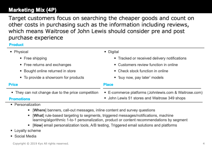
Although mobile payment users are 25% of British millenniums, more than 20% of them have tried and lapsed this method mainly via Apple Pay and Pingit which Barclays operated. This figure is relatively lower than EU countries, one of which is Italy having 37%. Therefore, Waitrose of John Lewis should adapt at least these two mobile platformers and PayPal (an existing non-bank financial brand) to improve CX. In addition, Pinterest is a less developed social media in comparison with other social channels primary Instagram. Thus, John Lewis can invest them to promote their products.
Customer Acquisition and Retention

The personalization, especially basket page can raise average order value (AOV). Therefore, this promotion can increase page not only views, conversion and retention rate but also AOV. However, the investment has to be commensurate with the cost, mainly acquisition one, the average of which for those who installed and registered on mobile shopping apps was totally $17.93 and those who made a purchase in 2019 was $39.38, which was almost half of 2017. On the other hand, AOV from a mobile phone was $ 86.47 in 2019 Q2. Thus, if this investment affect AOV negatively, it can be justified.
Reference
- Accenture, 2014. Accenture’s 2014 UK Financial Services Customer Survey.
- Adjust, 2019. Global mobile shopping app user acquisition costs 2017-2019. Statista [viewed 2 December 2019]. Available from: https://www.statista.com/statistics/1060743/mobile-shopping-apps-user-acquisition-cost-uk/
- Adjust, 2019. Mobile shopping apps user acquisition costs in the UK 2019. Statista [viewed 2 December 2019]. Available from: https://www.statista.com/statistics/1060743/mobile-shopping-apps-user-acquisition-cost-uk/
- Adjust, 2019. Mobile shopping apps: user acquisition rate in the UK 2019. Statista [viewed 2 December 2019]. Available from: https://www.statista.com/statistics/1060733/mobile-shopping-apps-user-acquisition-rate-uk/
- Deloitte, 2017. Bling it on What makes a millennial spend more.
- Eurostat, 2019. Population: Structure indicators [Online]. Available from: [http://appsso.eurostat.ec.europa.eu/nui/show.do?query=BOOKMARK_DS-054158QID_1E427F0_UID-3F171EB0&layout=TIME,C,X,0;GEO,L,Y,0;INDIC_DE,L,Z,0;INDICATORS,C,Z,1;&zSelection=DS-054158INDIC_DE,PC_Y2549;DS-054158INDICATORS,OBS_FLAG;&rankName1=INDICATORS_1_2-12&rankName2=INDIC-DE_1_2-12&rankName3=TIME_1_0_0_0&rankName4=GEO_1_2_0_1&sortC=ASC-1FIRST&rStp=&cStp=&rDCh=&cDCh=&rDM=true&cDM=true&footnes=false&empty=false&wai=false&time_mode=NONE&time_most_recent=false&lang=EN&cfo=%23%23%23%2C%23%23%23.%23%23%23](http://appsso.eurostat.ec.europa.eu/nui/show.do?query=BOOKMARK_DS-054158_QID_1E427F0_UID-3F171EB0&layout=TIME,C,X,0;GEO,L,Y,0;INDIC_DE,L,Z,0;INDICATORS,C,Z,1;&zSelection=DS-054158INDIC_DE,PC_Y2549;DS-054158INDICATORS,OBS_FLAG;&rankName1=INDICATORS_1_2-12&rankName2=INDIC-DE_1_2-12&rankName3=TIME_1_0_0_0&rankName4=GEO_1_2_0_1&sortC=ASC-1_FIRST&rStp=&cStp=&rDCh=&cDCh=&rDM=true&cDM=true&footnes=false&empty=false&wai=false&time_mode=NONE&time_most_recent=false&lang=EN&cfo=%23%23%23%2C%23%23%23.%23%23%23) [Accessed 2 December 2019].
- Experian, 2016. Millennial Me & My Money [Online]. Available from: https://www.experianplc.com/media/news/2016/millennial-me-my-money-jan-2016/ [Accessed 2 December 2019].
- Google, 2016. Google’s Omnichannel Customer Experience Review.
- Inviqa, 2017, What millennials want: online retail in the Amazon era.
- Ipsos MORI, 2019. Tech Tracker Q1 2019 Report.
- Ipsos MORI, 2016. THE MILLENNIAL INFLUENCE.
- JOHN LEWIS PARTNERSHIP PLC, 2018. NOW & THE FUTURE.
- JOHN LEWIS PARTNERSHIP PLC, 2019. Annual Report and Accounts 2019.
- KPMG, 2017. Retail Survey 2017 What consumers are telling us.
- Lyons, K., 2016. Generation Y: a guide to a much-maligned demographic [Online]. Available from: https://www.theguardian.com/world/2016/mar/07/millennials-generation-y-guide-to-much-maligned-demographic [Accessed 2 December 2019].
- MARKETLINE, 2019. John Lewis Partnership Plc [Online]. Available from: https://advantage.marketline.com/Company/Profile/john_lewis_partnership_plc?swot [Accessed 2 December 2019].
- Mixpanel, 2017. 2017 Product Benchmarks Report.
-
Monetate, 2018. Monetate Ecommerce Quarterly Report Q4 2018. - Monetate, 2019. Average value of global online shopping orders as of 2nd quarter 2019, by device (in U.S. dollars). Statista. Statista Inc. Accessed: November 29, 2019. Available from: https://www.statista.com/statistics/239247/global-online-shopping-order-values-by-device/ [Accessed 2 December 2019].
- Pitney Bowes, 2018. 2018 Global Ecommerce Study Summary Report.
- RESEARCHSCAPE INTERNATIONAL, 2018. 2018 Trends in Personalization.
- SimilarWeb.com, 2019. johnlewis.com October 2019 Overview [Online]. Available from: https://www.similarweb.com/website/johnlewis.com [Accessed 2 December 2019].
- SimilarWeb.com, 2019. waitrose.com October 2019 Overview [Online]. Available from: https://www.similarweb.com/website/waitrose.com [Accessed 2 December 2019].
- Statista, 2019. Internet usage demographics in the United Kingdom (UK). Statista [viewed 2 December 2019]. Available from: https://www.statista.com/study/23574/internet-usage-demographics-in-the-united-kingdom-statista-dossier/
- Statista, 2019. Statista dossier about e-commerce worldwide. Statista [viewed 2 December 2019]. Available from: https://www.statista.com/study/10653/e-commerce-worldwide-statista-dossier/
- Statista, 2019. Statista dossier on department stores in the United Kingdom (UK). Statista [viewed 2 December 2019]. Available from: https://www.statista.com/study/32423/department-stores-in-the-united-kingdom-uk-statista-dossier/
- Statista, 2019. Statista dossier on online grocery shopping among UK consumers. Statista [viewed 2 December 2019]. Available from: https://www.statista.com/study/39216/uk-consumers-online-grocery-shopping-statista-dossier/
- Statista, 2019. Statista dossier on the John Lewis Partnership plc in the United Kingdom (UK). Statista [viewed 2 December 2019]. Available from: https://www.statista.com/study/27327/john-lewis-partnership-statista-dossier/
- Summit, 2018. Summit ScorecardTop 50 UK Retailers’ Online Performance2018 Edition.
- VoucherCodes, RetailMeNot, France and WBR Insights, 2018. Retail perspectives and innovation: Payments, personalization and the phygital.
SALES FORECASTING
This is a modified version of the report for Business Analytics in Bath Full Time MBA Class of 2020.
SALES FORECASTING
Introduction
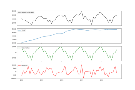
In this section, it is assumed and discussed that the recommended pizza will be added to the university catering service provider. The firm also can offer a variety of food lines mainly including sandwiches, wraps, crisps, salad and sushi meals. The supply chain management and cash-flow decisions of the company depend on one-month-ahead sales forecasting for 6 main meals. However, the current method to predict the demands can be primitive. This is primary because the monthly predictions have been done by the average of the last four month’s sales for each product with seasonal adjustments counted on their instinct. In addition, weekly demand estimation is simply done by the monthly one divided by four or five based on the number of days in the target month. Therefore, in section B, it is discussed how to improve one-month-ahead sales forecast. The data related to sales history for six of the main food lines is extracted which is divided by two part in terms of the amount of sales to analyze in Figure 12 and Figure 13 respectively. It is seen apparently most of food lines have a seasonality with the exception of ‘Wraps’ which might be almost constant.


Although there are several types of quantitative methods including time series and explanatory, the data will be analyzed by time series. One of the main reasons to do so is there is no other given explanatory data related to sales of food lines such as the size of market and share of that. This means each food line sales cannot be regressed to other factors. Therefore, time series analysis is suitable for the data. Time series analysis assume the observed data is the sum of three elements which are the trend (constant change), seasonality (cycle change) and noise (random change), which are shown in Figure 14 though Figure 19 (Downey, 2011).




There is a significant difference between stationary and non-stationary time series. This is because time series analysis also assumes the series is stationary which means no trend, no seasonality and the nature including amplitude and frequency of non-time varying noise (Janert, 2010). Hence, the assessment of the property plays the key role of the analysis. The autocorrelation value of stationary time series incline to decrease rapidly (Palachy, 2019). Autocorrelation means each data point is interacted with the succeeding one in the data (Downey, 2011). In addition, partial autocorrelation can reveal authentic correlation of a series and its lag with the exception of the one contributing from the intermediate lags (Prabhakaran, 2019). From Figure 20 to Figure 25 show autocorrelations of the sales of food lines seem to degrade relatively gradually which may mean these time series are non-stationary.


Other ways to asses stationary are statistical tests primary including ADF (Augmented Dickey Fuller) test and KPSS (Kwiatkowski-Phillips-Schmidt-Shin) test (SINGH, 2018). The null hypothesis of the former test is the time series obtains non-stationary which means if the P-Value is less than the significance level (0.05), the null hypothesis might be rejected (Prabhakaran, 2019). On the other hand, the null hypothesis of the latter test is reversed of the former (ibid). The result of ADF and KPSS test for the sales data of food lines are shown Figure 26 and Figure 27 respectively. Figure 26 shows P-Values are higher than 5% with the exception of ‘Wraps’, which means the time series of other food lines are likely to fail to reject null hypothesis and therefore they tend to be non-stationary. However, time series of ‘Wraps’ considerably inclined to reject null hypothesis and hence is likely to be stationary. One of main reasons to support the stationary of ‘Wraps’ sales is the null hypothesis is more likely to be rejected as ADF statistic value is more negative (Brownlee, 2016). Figure 27 demonstrates sales of ‘Crisps’ might be non-stationary due to the significance of P-Values (0.024 < 0.05). However, the remains tend to be stationary because their P-Values are not significant (rejected non-stationary hypothesis). There seems to be the contradictions between ADF test results and KPSS ones, however, there are the several types of stationarities which are strict stationary (the mean, variance and covariance do not depend on time), trend stationary (the equivalent of the strict one after removed a trend) and difference stationary (the equivalent of the strict one after differencing) (SINGH, 2018). In addition, KPSS test can categorize strict stationary or trend stationary and ADF test is also known as a difference stationarity test (ibid).


As a result of introducing the type of stationary, the sales of food lines can be separated as strict stationary, trend one and non-stationary (See Figure 28).

However, stationary is required to improve the accuracy of the prediction due to the fact that time series modeling supposed to be so as a fundamental assumption. There is some method to transform the series (strict) stationary such as taking the logarithm, differencing and removing rolling average (Prabhakaran, 2019). In fact, the differencing the sales of ‘Crisps’ seems to obtain strict stationary with ADF statistic value -7.230 (P-Value 0.000) and KPSS statistic value 0.136 (P-Value 0.100), which mean both tests might reject nonstationary hypothesis. Hence, after executed the differentiation for other non-strict stationary, they might have strict stationary except the sales of ‘Salad’, which are shown in Figure 29 and Figure 30.


Instead of differencing, removing 9 month moving average for the sales of ‘Salad’, it is more likely to possess strict stationary with ADF statistic value -4.506 (P-Value 0.000) and KPSS statistic value 0.304 (P-Value 0.100). As a result of some transformations, more forecastable time series are obtained.
Box–Jenkins Method
ARIMA
There are several forecast models for the time series mainly including autoregressive integrated moving average (ARIMA) model. ARIMA is a forecast model based on the past data, its lags and the lagged error, which is determined by three factors that are the minimum number of differencing required to transform the series stationary (‘d’), the number of lags of the data to be employed as forecasters (‘p’) and the number of lagged estimated errors (‘q’) (ibid). As it has shown, all series can be transformed to strict stationary one and therefore these might be modeled by ARIMA. The parameters (p, q, d) were calibrated by minimizing Akaike Information Criteria (AIC) which is one of the common criteria to find the best model ones and it means the lower is better seen in Figure 31 (Prabhakaran, 2019).

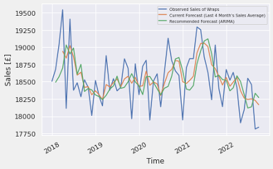
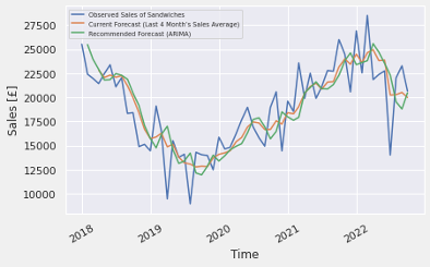
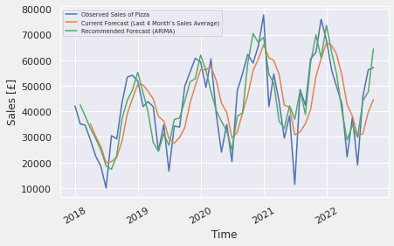
Figure 32 though 37 visualizes the estimated data in comparison with the observed one and the average of the last 4 month’s sales for the one. It seems to relatively capture the features of the series such as trend and cycle in comparison with the current forecasting method, however, still the comparably differences between them are remained.


SARIMAX
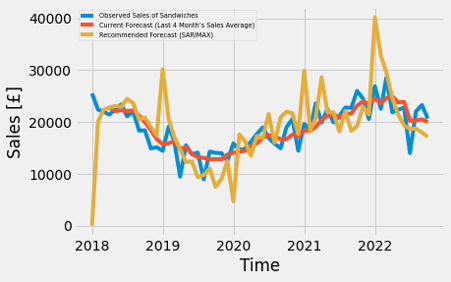
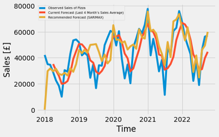
Seasonal Autoregressive Integrated Moving-Average with Exogenous Regressors (SARIMAX) can be the well-known natural extension of ARIMA, which may improve the predictability further to adapt seasonal differencing that deduct the value from preceding season (ibid). The best parameters including seasonal modeling ones (added bar s after the name of ARIMA ones to distinguish them) are selected in the certain range as they have the lowest AIC in Figure 38.

However, the outcomes of modeling (shown in Figure 39 through Figure 44) might not suitable for the sales date of food lines due to the fact that it seems to overestimate the seasonality. This may mean the more complex and lower AIC model do not lead to the higher accuracy of the prediction. Therefore, it is required to adapt time series into another framework for the further improvement.



State Space Model
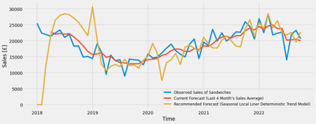
One of the best alternatives of Box–Jenkins approach such as ARIMA can be state space models (Meulman and Koopman, 2007). It formulates the unobserved dynamic process (state) of time series, which can divide a several components such as deterministic (or stochastic) level, slope and seasonal, therefore, they are individually formulated and estimated (ibid). Although there are several state space models, the best fit models are determined by the lowest AIC which is shown in Figure 45. Figure 46 through 51 demonstrate the comparison observed data, current forecast (4 months moving average) and the best fit liner state space model. It can be seen state space model might be able to predict more accuracy than ARIMA models with exception of the eldest year (2018-2019).




The Prophet Forecasting Model
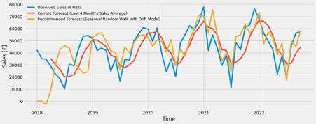
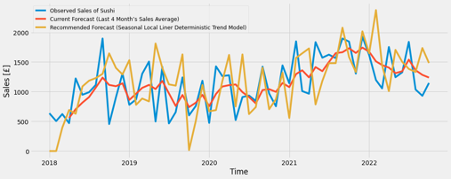
Another type of mothed can be Prophet which is developed by Facebook for time series analysis (Taylor and Letham, 2017). This model estimates the trend of time series by extending the generalized additive model which is a class of regression models and do so the seasonality by Fourier series, the parameters of which are calibrated by AIC automatically (ibid). The result seen in Figure 52 through 57 seem to predict more feasible than ARIMA and state space model with exception of the latest year (after the late of 2021).


LSTM RNN
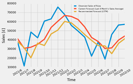
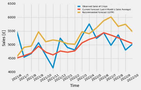
One of the major alternatives to rise the predictability of time series can be Long Short-Term Memory network (LSTM). It is a specialized layer of Recurrent Neural Network (RNN) that is more suitable for time series than other type of NN to manage an internal state encapsulating the data seen earlier (TensorFlow, 2020). The architecture of LSTM RNN used for sales predictions of food lines is seen in Figure 58, which has the input shape, which is 3-time step with 1 feature, 100 neurons in LSTM layer, dropout 50% and a Dense output layer with 1 neuron. It is also used the Mean Absolute Error (MAE) loss function and RMSprop as an optimization algorithm to fit for 1000 training epochs with a batch size of 1. It is trained by 67% of the data and the remains are used for the predictions. The forecast by LSTM RNN (seen in Figure 59 through Figure 64) show it tends to underestimate the amount of sales in the reason of forecast period (the latest 17 months).




Comparison
Mean Square Error (MSE) can be one of the most common method to compare the model accuracy. Figure 65 demonstrates MSEs of the models, the parameters of which are chosen by the lowest AIC. It can be seen the most accurate model might depend on the food lines, for example, ARIMA model should be selected if it is required to forecast the sales of ‘Salad’ because it lead to the lowest MSE, however, as for ‘Sushi’ and ‘Crisps’, LSTM model is preferable. In addition, Prophet model is recommended if the objective of sales predictions is ‘Wraps’, ‘Sandwiches’ and ‘Crisps’.

Reference
- Brownlee, J., 2016. How to Check if Time Series Data is Stationary with Python [Online]. Available from: https://machinelearningmastery.com/time-series-data-stationary-python/ [Accessed 30 March 2020].
- Brownlee, J., 2017. Long Short-Term Memory Networks with Python
- Downey, A.B., 2011. Think Stats
- Janert, P.K., 2010. Data Analysis with Open Source Tools
- Janssens, W., Wijnen, K., Pelsmacker, P.D., Kenhove, P.V., 2008. Marketing Research with SPSS (FT Prentice Hall)
- Lilien, G.L. and Rangaswamy, A., 2002. Marketing Engineering: Computer Assisted Marketing Analysis and Planning
- Meulman, J.J. and Koopman, S.J., 2007. An Introduction to State Space Time Series Analysis
- Palachy, S., 2019. Detecting stationarity in time series data [Online]. Available from: https://towardsdatascience.com/detecting-stationarity-in-time-series-data-d29e0a21e638 [Accessed 30 March 2020].
- Prabhakaran, S., 2019. ARIMA Model – Complete Guide to Time Series Forecasting in Python [Online]. Available from: https://www.machinelearningplus.com/time-series/arima-model-time-series-forecasting-python/ [Accessed 30 March 2020].
- Prabhakaran, S., 2019. Time Series Analysis in Python – A Comprehensive Guide with Examples [Online]. Available from: https://www.machinelearningplus.com/time-series/time-series-analysis-python/ [Accessed 30 March 2020].
- SINGH, A., 2018. A Gentle Introduction to Handling a Non-Stationary Time Series in Python [Online]. Available from: https://www.analyticsvidhya.com/blog/2018/09/non-stationary-time-series-python/ [Accessed 30 March 2020].
- Taylor, S.J. and Letham, B., 2017. Forecasting at scale. PeerJ Preprints 5:e3190v2 https://doi.org/10.7287/peerj.preprints.3190v2
- TensorFlow, 2020. Time series forecasting [Online]. Available from: https://www.tensorflow.org/tutorials/structured_data/time_series [Accessed 30 March 2020].
- Tieleman, T. and Hinton, G., 2012. Lecture 6.5-rmsprop: Divide the Gradient by a Running Average of Its Recent Magnitude. COURSERA: Neural Networks for Machine Learning, 4, 26-31.
- Wierenga, B., 2008. Handbook of Marketing Decision Models