SALES FORECASTING
This is a modified version of the report for Business Analyics in Bath Full Time MBA Class of 2020.
SALES FORECASTING
Introduction
In this section, it is assumed and discussed that the recommended pizza will be added to the university catering service provider. The firm also can offer a variety of food lines mainly including sandwiches, wraps, crisps, salad and sushi meals. The supply chain management and cash-flow decisions of the company depend on one-month-ahead sales forecasting for 6 main meals. However, the current method to predict the demands can be primitive. This is primary because the monthly predictions have been done by the average of the last four month’s sales for each product with seasonal adjustments counted on their instinct. In addition, weekly demand estimation is simply done by the monthly one divided by four or five based on the number of days in the target month. Therefore, in section B, it is discussed how to improve one-month-ahead sales forecast. The data related to sales history for six of the main food lines is extracted which is divided by two part in terms of the amount of sales to analyze in Figure 12 and Figure 13 respectively. It is seen apparently most of food lines have a seasonality with the exception of ‘Wraps’ which might be almost constant.


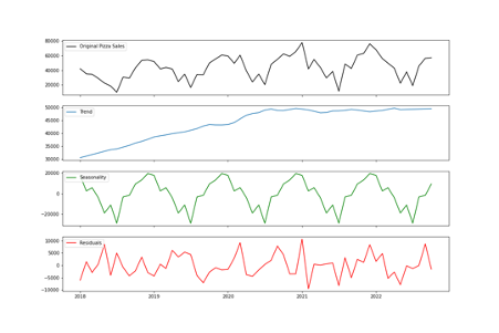
Although there are several types of quantitative methods including time series and explanatory, the data will be analyzed by time series. One of the main reasons to do so is there is no other given explanatory data related to sales of food lines such as the size of market and share of that. This means each food line sales cannot be regressed to other factors. Therefore, time series analysis is suitable for the data. Time series analysis assume the observed data is the sum of three elements which are the trend (constant change), seasonality (cycle change) and noise (random change), which are shown in Figure 14 though Figure 19 (Downey, 2011).




There is a significant difference between stationary and non-stationary time series. This is because time series analysis also assumes the series is stationary which means no trend, no seasonality and the nature including amplitude and frequency of non-time varying noise (Janert, 2010). Hence, the assessment of the property plays the key role of the analysis. The autocorrelation value of stationary time series incline to decrease rapidly (Palachy, 2019). Autocorrelation means each data point is interacted with the succeeding one in the data (Downey, 2011). In addition, partial autocorrelation can reveal authentic correlation of a series and its lag with the exception of the one contributing from the intermediate lags (Prabhakaran, 2019). From Figure 20 to Figure 25 show autocorrelations of the sales of food lines seem to degrade relatively gradually which may mean these time series are non-stationary.


Other ways to asses stationary are statistical tests primary including ADF (Augmented Dickey Fuller) test and KPSS (Kwiatkowski-Phillips-Schmidt-Shin) test (SINGH, 2018). The null hypothesis of the former test is the time series obtains non-stationary which means if the P-Value is less than the significance level (0.05), the null hypothesis might be rejected (Prabhakaran, 2019). On the other hand, the null hypothesis of the latter test is reversed of the former (ibid). The result of ADF and KPSS test for the sales data of food lines are shown Figure 26 and Figure 27 respectively. Figure 26 shows P-Values are higher than 5% with the exception of ‘Wraps’, which means the time series of other food lines are likely to fail to reject null hypothesis and therefore they tend to be non-stationary. However, time series of ‘Wraps’ considerably inclined to reject null hypothesis and hence is likely to be stationary. One of main reasons to support the stationary of ‘Wraps’ sales is the null hypothesis is more likely to be rejected as ADF statistic value is more negative (Brownlee, 2016). Figure 27 demonstrates sales of ‘Crisps’ might be non-stationary due to the significance of P-Values (0.024 < 0.05). However, the remains tend to be stationary because their P-Values are not significant (rejected non-stationary hypothesis). There seems to be the contradictions between ADF test results and KPSS ones, however, there are the several types of stationarities which are strict stationary (the mean, variance and covariance do not depend on time), trend stationary (the equivalent of the strict one after removed a trend) and difference stationary (the equivalent of the strict one after differencing) (SINGH, 2018). In addition, KPSS test can categorize strict stationary or trend stationary and ADF test is also known as a difference stationarity test (ibid).


As a result of introducing the type of stationary, the sales of food lines can be separated as strict stationary, trend one and non-stationary (See Figure 28).

However, stationary is required to improve the accuracy of the prediction due to the fact that time series modeling supposed to be so as a fundamental assumption. There is some method to transform the series (strict) stationary such as taking the logarithm, differencing and removing rolling average (Prabhakaran, 2019). In fact, the differencing the sales of ‘Crisps’ seems to obtain strict stationary with ADF statistic value -7.230 (P-Value 0.000) and KPSS statistic value 0.136 (P-Value 0.100), which mean both tests might reject nonstationary hypothesis. Hence, after executed the differentiation for other non-strict stationary, they might have strict stationary except the sales of ‘Salad’, which are shown in Figure 29 and Figure 30.


Instead of differencing, removing 9 month moving average for the sales of ‘Salad’, it is more likely to possess strict stationary with ADF statistic value -4.506 (P-Value 0.000) and KPSS statistic value 0.304 (P-Value 0.100). As a result of some transformations, more forecastable time series are obtained.
Box–Jenkins Method
ARIMA
There are several forecast models for the time series mainly including autoregressive integrated moving average (ARIMA) model. ARIMA is a forecast model based on the past data, its lags and the lagged error, which is determined by three factors that are the minimum number of differencing required to transform the series stationary (‘d’), the number of lags of the data to be employed as forecasters (‘p’) and the number of lagged estimated errors (‘q’) (ibid). As it has shown, all series can be transformed to strict stationary one and therefore these might be modeled by ARIMA. The parameters (p, q, d) were calibrated by minimizing Akaike Information Criteria (AIC) which is one of the common criteria to find the best model ones and it means the lower is better seen in Figure 31 (Prabhakaran, 2019).

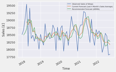
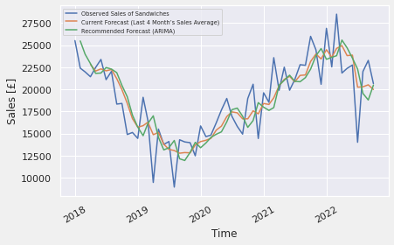
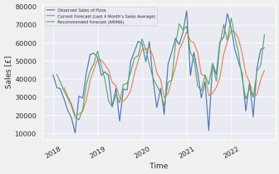
Figure 32 though 37 visualizes the estimated data in comparison with the observed one and the average of the last 4 month’s sales for the one. It seems to relatively capture the features of the series such as trend and cycle in comparison with the current forecasting method, however, still the comparably differences between them are remained.


SARIMAX
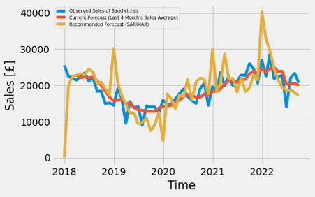
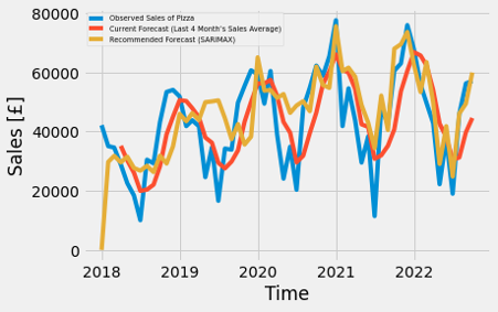
Seasonal Autoregressive Integrated Moving-Average with Exogenous Regressors (SARIMAX) can be the well-known natural extension of ARIMA, which may improve the predictability further to adapt seasonal differencing that deduct the value from preceding season (ibid). The best parameters including seasonal modeling ones (added bar s after the name of ARIMA ones to distinguish them) are selected in the certain range as they have the lowest AIC in Figure 38.

However, the outcomes of modeling (shown in Figure 39 through Figure 44) might not suitable for the sales date of food lines due to the fact that it seems to overestimate the seasonality. This may mean the more complex and lower AIC model do not lead to the higher accuracy of the prediction. Therefore, it is required to adapt time series into another framework for the further improvement.



State Space Model
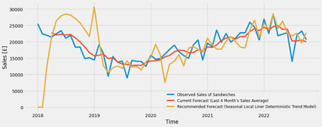
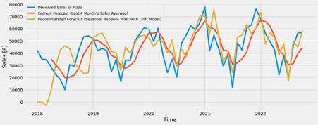
One of the best alternatives of Box–Jenkins approach such as ARIMA can be state space models (Meulman and Koopman, 2007). It formulates the unobserved dynamic process (state) of time series, which can divide a several components such as deterministic (or stochastic) level, slope and seasonal, therefore, they are individually formulated and estimated (ibid). Although there are several state space models, the best fit models are determined by the lowest AIC which is shown in Figure 45. Figure 46 through 51 demonstrate the comparison observed data, current forecast (4 months moving average) and the best fit liner state space model. It can be seen state space model might be able to predict more accuracy than ARIMA models with exception of the eldest year (2018-2019).




The Prophet Forecasting Model
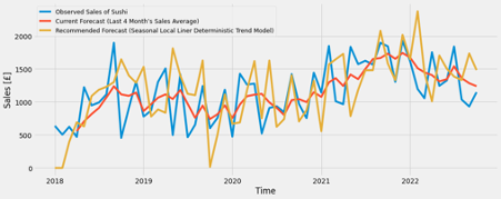
Another type of mothed can be Prophet which is developed by Facebook for time series analysis (Taylor and Letham, 2017). This model estimates the trend of time series by extending the generalized additive model which is a class of regression models and do so the seasonality by Fourier series, the parameters of which are calibrated by AIC automatically (ibid). The result seen in Figure 52 through 57 seem to predict more feasible than ARIMA and state space model with exception of the latest year (after the late of 2021).


LSTM RNN
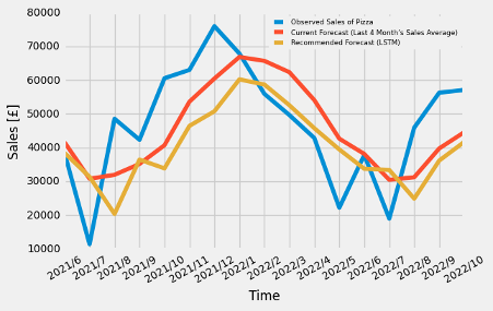
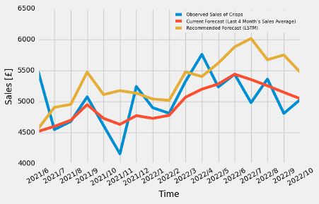
One of the major alternatives to rise the predictability of time series can be Long Short-Term Memory network (LSTM). It is a specialized layer of Recurrent Neural Network (RNN) that is more suitable for time series than other type of NN to manage an internal state encapsulating the data seen earlier (TensorFlow, 2020). The architecture of LSTM RNN used for sales predictions of food lines is seen in Figure 58, which has the input shape, which is 3-time step with 1 feature, 100 neurons in LSTM layer, dropout 50% and a Dense output layer with 1 neuron. It is also used the Mean Absolute Error (MAE) loss function and RMSprop as an optimization algorithm to fit for 1000 training epochs with a batch size of 1. It is trained by 67% of the data and the remains are used for the predictions. The forecast by LSTM RNN (seen in Figure 59 through Figure 64) show it tends to underestimate the amount of sales in the reason of forecast period (the latest 17 months).




Comparison
Mean Square Error (MSE) can be one of the most common method to compare the model accuracy. Figure 65 demonstrates MSEs of the models, the parameters of which are chosen by the lowest AIC. It can be seen the most accurate model might depend on the food lines, for example, ARIMA model should be selected if it is required to forecast the sales of ‘Salad’ because it lead to the lowest MSE, however, as for ‘Sushi’ and ‘Crisps’, LSTM model is preferable. In addition, Prophet model is recommended if the objective of sales predictions is ‘Wraps’, ‘Sandwiches’ and ‘Crisps’.

Reference
- Brownlee, J., 2016. How to Check if Time Series Data is Stationary with Python [Online]. Available from: https://machinelearningmastery.com/time-series-data-stationary-python/ [Accessed 30 March 2020].
- Brownlee, J., 2017. Long Short-Term Memory Networks with Python
- Downey, A.B., 2011. Think Stats
- Janert, P.K., 2010. Data Analysis with Open Source Tools
- Janssens, W., Wijnen, K., Pelsmacker, P.D., Kenhove, P.V., 2008. Marketing Research with SPSS (FT Prentice Hall)
- Lilien, G.L. and Rangaswamy, A., 2002. Marketing Engineering: Computer Assisted Marketing Analysis and Planning
- Meulman, J.J. and Koopman, S.J., 2007. An Introduction to State Space Time Series Analysis
- Palachy, S., 2019. Detecting stationarity in time series data [Online]. Available from: https://towardsdatascience.com/detecting-stationarity-in-time-series-data-d29e0a21e638 [Accessed 30 March 2020].
- Prabhakaran, S., 2019. ARIMA Model – Complete Guide to Time Series Forecasting in Python [Online]. Available from: https://www.machinelearningplus.com/time-series/arima-model-time-series-forecasting-python/ [Accessed 30 March 2020].
- Prabhakaran, S., 2019. Time Series Analysis in Python – A Comprehensive Guide with Examples [Online]. Available from: https://www.machinelearningplus.com/time-series/time-series-analysis-python/ [Accessed 30 March 2020].
- SINGH, A., 2018. A Gentle Introduction to Handling a Non-Stationary Time Series in Python [Online]. Available from: https://www.analyticsvidhya.com/blog/2018/09/non-stationary-time-series-python/ [Accessed 30 March 2020].
- Taylor, S.J. and Letham, B., 2017. Forecasting at scale. PeerJ Preprints 5:e3190v2 https://doi.org/10.7287/peerj.preprints.3190v2
- TensorFlow, 2020. Time series forecasting [Online]. Available from: https://www.tensorflow.org/tutorials/structured_data/time_series [Accessed 30 March 2020].
- Tieleman, T. and Hinton, G., 2012. Lecture 6.5-rmsprop: Divide the Gradient by a Running Average of Its Recent Magnitude. COURSERA: Neural Networks for Machine Learning, 4, 26-31.
- Wierenga, B., 2008. Handbook of Marketing Decision Models
Related Posts
- SALES FORECASTING 2
- Organize and implement Hull and White (1994a) interest rate model
- Derivation of Black-Scholes PDE and its analytical solution by arbitrage pricing theory
- Derivation of yield curve construction formula with tenor basis spread
- Venture capital finance
- Strategic brand management
- Sources of finance