SALES FORECASTING 2
This is a modified version of the report for Business Analyics in Bath Full Time MBA Class of 2020.
SALES FORECASTING 2
Introduction
In this section, it is assumed a pizza parlor business plan in the Bath University has lunched. The vital issue of the plan is also done so to find one or two pizzas which might be appealed by the Bath University students based on the attributions such as type of topping and base. Hence, it will be conducted an experiment to attempt diverse pizzas for the target consumers including the students. However, there are some constrictions for the plan, one of which is the maximum budget of £100 to purchase the pizzas for this experiment. One of the major tools to find the customer preferences can be conjoint analysis which assumed their preferences as a combination of the attributions having a certain degree (Janssens et al., 2008). Therefore, it should be decided that which attributions might be the most relevant to the purpose that is to find the most preferred among the students. The consideration relevant to the attributions was started from the research suggesting 5 attributions which are the crust, topping, cheese type, cheese quality and price (Lilien and Rangaswamy, 2002). The crust has 3 levels which are thin, thick, pan. Topping’s levels are pineapple, veggie, chicken, turkey. The levels of cheese type are Romano, mixed, mozzarella. These of cheese quality are 50g, 75g, 100g. £4.99, £6.99, £8.99 are the level of price. As a result, the total possible combinations of attribute levels are 324 (= 3 x 4 x 3 x 3 x 3). All of them cannot be conducted due to the time and budget restrictions, however, some researchers argued the effective number of part worth parameters to be approximated from conjoint data, the number of which is less than the sum of all levels of each attribution (Wierenga, 2008). Thus, if at most 16 (= 3 + 4 + 3 + 3 + 3) candidates are selected precisely, these alternatives can be represented all of the possible combinations of attribute levels (ibid). The selection usually is done by SPSS from all of attribute levels and therefore, the data format to save 16 alternatives representing all possibilities should be suitable for the application. Furthermore, the data structure of that should be 16 rows with at least 7 columns which are 5 attributions, the primary key and the preference score. The most well-liked pizza should the maximum preference score (one hundred) and the minimum one (zero) should be rated to the least popular pizza. Hence. Each pizza must have the preference score from 0 to 100. Conjoint analysis assumes the preference score can be represented the weighted sum of the utilities for each attribution (Wierenga, 2008). This means after collecting the score from the customers being tested, the software (SPSS) can discover weights and utilities of each attributions. In addition, the key is required to identify each rows, however, it is automatically inserted (see the leftist column of figure 1) when the data is inputted in the data format and then also accordingly the column named ‘STATUS’ with ‘Design’ as the value is inserted as a result of using the function to generate the orthogonal design (Janssens et al., 2008).
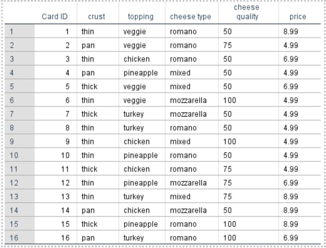
Furthermore, although it should be tested 16 type of pizzas to collect the target customer preference as the score, there is the budged limitation which the pizzas only can be purchased less than 100 pounds. This means if assumed the price of normal size pizza is 15 pounds, 6 pizzas are able to be bought for the experiment. Supposed the shop selected to buy the pizzas can allow to consume at least 3 type of the alternatives among 16 of that in the same pizza, 18 different type of pizza is available for the test. Therefore, all of alternatives are able to be examined with only 2 duplicates (16 = 18 - 2). Because of the fact that 6 students are applicable for the evaluation, if each student can eat and rate all of alternatives to cut each piece into 6 parts, the preferable scores of them are able to be collected. Figure 2 is assumed the result of the 16 alternative pizzas rating by 6 students (identified by id in the figure). For instance, the column named ‘sco1’ means the students (identified by id in the figure 2) rating score for the top row in the figure 1 (Card ID 1 row).

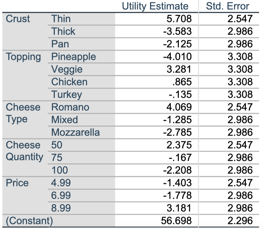
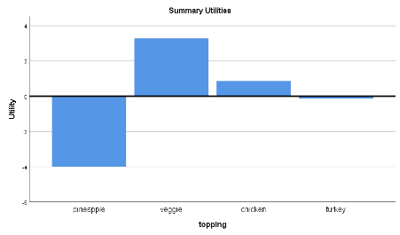
The utilities of each attributions are estimated by the software, SPSS. In Figure 3, it is seen apparently that the attribution ‘thin’ (assigned to ‘Crust’ level) has the highest utility (5.708) and the lowest utility (-4.010) is earned by the attribution ‘pineapple’ (belonged to ‘Topping’ level). Utilities
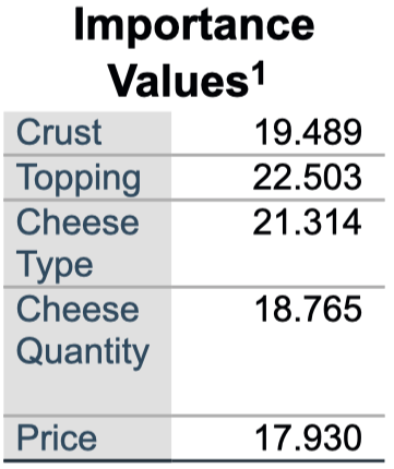
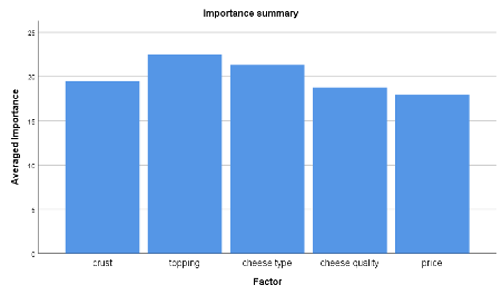
In addition, Figure 4 shows the averaged importance for each levels of the attributions which mean which levels can earn the highest utility. In the figure, the level ‘Topping’ has the highest one (22.503) and the lowest one (17.930) is gained by the level ‘Price’.
Furthermore, Figure 5 indicates that both the Pearson’s R (.864) and the Kendall’s tau (.639) which mean the correlations between the recognized and forecasted preferences are high (ibid). both correlations also are likely to be significant (respectively .000 and .000) because less than .05 significance means the null hypothesis of a null correlation is quite unlikely to be acceptable (ibid). Correlations2

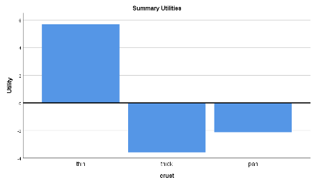
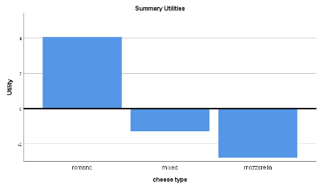
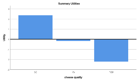
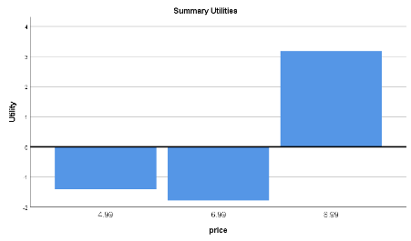
Finally, Figures 6 through 10, the relative utility levels are demonstrated for each attribute and In Figure 11, the mean importance is displayed for each attribute (ibid). From Figures 6 through 11, it could be seen that the pizza parlor that offers their customers a thin of crust, Veggie of topping, Romano of cheese type, 50g of cheese quantity and pricing £8.99 might achieve the highest utility.
Reference
- Brownlee, J., 2016. How to Check if Time Series Data is Stationary with Python [Online]. Available from: https://machinelearningmastery.com/time-series-data-stationary-python/ [Accessed 30 March 2020].
- Brownlee, J., 2017. Long Short-Term Memory Networks with Python
- Downey, A.B., 2011. Think Stats
- Janert, P.K., 2010. Data Analysis with Open Source Tools
- Janssens, W., Wijnen, K., Pelsmacker, P.D., Kenhove, P.V., 2008. Marketing Research with SPSS (FT Prentice Hall)
- Lilien, G.L. and Rangaswamy, A., 2002. Marketing Engineering: Computer Assisted Marketing Analysis and Planning
- Meulman, J.J. and Koopman, S.J., 2007. An Introduction to State Space Time Series Analysis
- Palachy, S., 2019. Detecting stationarity in time series data [Online]. Available from: https://towardsdatascience.com/detecting-stationarity-in-time-series-data-d29e0a21e638 [Accessed 30 March 2020].
- Prabhakaran, S., 2019. ARIMA Model – Complete Guide to Time Series Forecasting in Python [Online]. Available from: https://www.machinelearningplus.com/time-series/arima-model-time-series-forecasting-python/ [Accessed 30 March 2020].
- Prabhakaran, S., 2019. Time Series Analysis in Python – A Comprehensive Guide with Examples [Online]. Available from: https://www.machinelearningplus.com/time-series/time-series-analysis-python/ [Accessed 30 March 2020].
- SINGH, A., 2018. A Gentle Introduction to Handling a Non-Stationary Time Series in Python [Online]. Available from: https://www.analyticsvidhya.com/blog/2018/09/non-stationary-time-series-python/ [Accessed 30 March 2020].
- Taylor, S.J. and Letham, B., 2017. Forecasting at scale. PeerJ Preprints 5:e3190v2 https://doi.org/10.7287/peerj.preprints.3190v2
- TensorFlow, 2020. Time series forecasting [Online]. Available from: https://www.tensorflow.org/tutorials/structured_data/time_series [Accessed 30 March 2020].
- Tieleman, T. and Hinton, G., 2012. Lecture 6.5-rmsprop: Divide the Gradient by a Running Average of Its Recent Magnitude. COURSERA: Neural Networks for Machine Learning, 4, 26-31.
- Wierenga, B., 2008. Handbook of Marketing Decision Models
Related Posts
- Organize and implement Hull and White (1994a) interest rate model
- Derivation of Black-Scholes PDE and its analytical solution by arbitrage pricing theory
- Derivation of yield curve construction formula with tenor basis spread
- Venture capital finance
- Strategic brand management
- Sources of finance
- Knowledge Leadership in a Global Economy